Interpreting Yield Results – Data Variability and Evaluation
September 25, 2023
- Even the most superior seed products do not win yield comparisons in every plot.
- It is important to understand plot yield data and why a high-yielding product with the best average yield across multiple locations does not have the highest yield at every location.
- Yield data may change as the harvest season progresses and more trials are included in an overall average.
Measured yield performance of any product is the result of the genetics (G) of the product and the environment (E) in which it is tested, with the combined effects known as the G x E interaction. One must always keep in mind that yield trials deal with many variables that can contribute to yield performance. Average yields can also change as more data is accumulated across locations. Greater quantities of yield data will likely give a clearer picture of the actual yield potential.
Variability of Observations is a Natural Thing
Most genetic traits that contribute to yield are quantitative traits, which means they are controlled by multiple genes that each contribute a certain percentage to the overall trait. Observations of any quantitative trait, such as height of an individual or yield for a plot or strip trial, usually follow a bell-shaped curve (Figure 1). This variation is due to the G x E interaction, as the environment can have independent and different effects on each of the genes contributing to the expression of the trait. Most observations are close to the mean (average), but some observations—usually 5% or less—appear to be very different from the mean. These values are not wrong or incorrect, but just part of the natural variation seen in any data set. For example, consider height for men in the United States. If the average height is 70 inches, most men will be between 66 and 74 inches tall, but a few will be much taller, and a few others will be much shorter. Yield—and most other quantitative measurements of any particular trait—will follow a similar pattern.
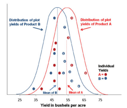
As illustrated in Figure 1, the means of Product A and Product B are different. However, there is overlap between the two products. You can see that an individual measurement for Product B may be higher than Product A even though the overall mean of Product A is higher.
This higher measurement for Product B may be a response to the specific environment, or it may just be due to chance. Some environments may favor one product over another, resulting in a higher plot yield for Product B than for Product A even though Product A is the better overall performer. Environmental factors such as excess moisture, drought, or disease may favor Product B, while in a different environment the opposite might be true based on Product A’s and Product B’s responses to their environment. Some differences may also be due to experimental error.
The Importance of Having All the Data
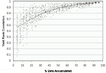
Because of the inherent variability that occurs in biological systems, the initial data that is reported may not give a clear picture of the actual average performance of a product. Figure 2 charts the percent accumulated data against the rank correlations among entries in a yield plot. As harvest season begins and limited field data is collected, the correlation is low (left side of the graph area, Figure 2). As the harvest season progresses and yield data accumulates, the correlation becomes stronger and moves closer to a value of 1, with a value of 1 here representing that the true mean yield potential has been determined with 100% certainty. By the end of the harvest season, the correlation increases dramatically to over 90% (0.9 on the vertical axis, Figure 2) as the large quantity of accumulated data gives a better estimate of the yield potential of a product and its rank among the other field plot entries. Thus, with very little data accumulated, the rankings of various products within the yield plot when compared to rankings across other plots can be extremely variable. As the data is accumulated over time, how a particular product will rank in the plot will likely become more consistent and provide a better estimate of the true yield potential.
The more data that is accumulated on a given product, the more stable its ranking among multiple products becomes. In the example in Figure 1, there are eleven individual yield data points of each product, and all values are within their given distributions of the true mean yield. However, within this limited data set, seven of the eleven individual yields of Product B are closely centered or greater than the true mean yield of Product A, while only four out of eleven individual yields of Product A are greater or centered around its own true mean. While the actual mean of Product A will be greater than Product B once all the data is collected, as shown by the position of the dotted line, it would initially appear that Product B is the higher yielder based on a limited, early data set.
It is also important that when comparing products across multiple testing locations, that all the products are represented an equal number of times. For example, you may be interested in comparing the average performance of Products A, B, C and D, and you have yield results from a total of ten plot locations in your local area. If Product A appeared in only eight of the 10 trials while the Products B, C and D appeared at all 10, the data is not balanced. This unbalanced data could lead to erroneous conclusions about the performance of Product A.
Yield Stability Across Various Soil Types and Environments
As has been previously mentioned, environment (i.e., soil type, climate, irrigated or rainfed, etc.) is one of the two primary factors driving product performance relative to other products. Some products perform well in lighter-textured soil, some do not. Some perform well regardless of soil type. Placing a strip trial within a uniform soil texture is important, although with modern day yield mapping capabilities doing so has become less of an issue. However, soil texture is an example of one factor to take into consideration when selecting products. If you do not have any light-textured soil on your farm, you may not want to consider yield trials that were conducted in soils with a high percentage of sand when evaluating product performance. A certain product may have good drought tolerance which enhances its adaptation to low- or moderate-yield environments such as rainfed fields but may not be as competitive in higher-yield environments such as irrigated fields or those with high water-holding capacity.
Rolling the Test-Plot Dice
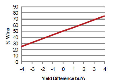
Probability is another factor in determining the winner in a test plot. The chance of a product winning depends on how many other products it is compared to in the trial, the relative difference in their yields, or the superiority of one product over another. If two products have equal yield potential, the odds of either one wining are like the 50:50 odds of head or tails when you toss a coin. If you toss a coin 10 times, you may get six heads and four tails instead of five heads and five tails, but the two outcomes are not actually significantly different. The same is true of a field trial. If two products are equal in yield potential, the odds of either one wining are 50%. If one product is superior, it will win more frequently, but a win is still not assured in every test. Figure 3 shows an example based on soybean data. Note that even if a product has a four bu/acre overall yield advantage, it will likely win only 75% of the head-to-head comparisons in a yield plot. Conversely the product that is actually four bushels less can still win 25% of the time.
Statistics 101
A statistically significant result signifies that the results are unlikely to have occurred by chance and have a high probability of being a true difference caused by trial conditions, and thus of being repeatable. If yield differences are not determined to be statistically significant, it indicates that the differences due to seed products (or other treatments) are not large enough relative to the experimental variation in the field, and that any differences are likely the result of random chance, just as when ten coinflips produce six heads and four tails.
Statistical significance is related to a number that often appears in research graphs or tables called a probability value, or p-value. This value assists in determining if the differences that are detected in a field trial are due to random error or to the treatment (e.g., seed product, fertilizer application rates, herbicide products, etc.). A common p-value for on-farm research trials is 10% (or p = 0.10). A p-value of 0.10 indicates that there is a 10% chance that any statistically significant difference among treatments is due to random chance, and a 90% chance that significant differences are due to the treatment.
Another number that university and independent plot results may include is an LSD, which stands for least significant difference. The LSD indicates the amount of yield variation that can be attributed to the product itself versus influence from outside factors. Yield differences greater than the LSD can be attributed to actual differences in genetic yield potentials of products. Yield differences less than the LSD are not considered statistically significant and are likely due to outside factors. An example is given in Table 1. Often, you will find the LSD at the bottom of the yield table in performance trial results.
Table 1. Least Significant Difference Example.
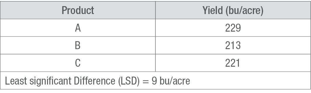
Table 1 is example data from a hypothetical university field trial whose LSD was 9 at a significance level of p = 0.10. The difference in yield between products A and B is 16 bu/acre. Because 16 is greater than the LSD of 9, we are 90% confident that the yield level is indeed significantly different and not likely due to experimental variation in the field or random chance, but to genetic differences. The difference in yield between products B and C is 8 bu/acre. Because 8 is less than the LSD of 9, we cannot conclude that the yield levels are significantly different, and the difference is likely due to experimental variation in the field or random chance, and not to genetic differences.
Summary
No product, even if it is truly superior, will win every yield plot. Over many tests, industry-leading products have typical head-to-head winning percentages of only 60 to 65%. Environmental factors, genetic potential, and test site variability constitute the variables that primarily contribute to yield differences across test plot sites. Yield ranks among entries in complied data sets can also change based on the number of tests and the geographical location of the plots. The more data and comparisons that are collected, the better the picture of yield performance. A more robust data set can increase the degree of confidence in picking a winning product.
1110_298901
Disclaimer
ALWAYS READ AND FOLLOW GRAIN MARKETING AND ALL OTHER STEWARDSHIP PRACTICES AND PESTICIDE LABEL DIRECTIONS.